• home
• writing
• research

Models of synaptic conductance I

NOTE  In this set of articles I would like to cover three simple models of synaptic conductance which are typically used in spiking networks. While people are quite familiar with their general logic, the exact mathematical details are often overlooked or simply swept under the rug because they are deemed too simple. I will take on this all-too-simple task, and talk about the mathematical ideas behind these basic models.

When a pre-synaptic neurone emits a spike, the transfer function across its synapses dictates how electric flux (charge) flows into its post-synaptic partners. This transfer function can be modelled to various degrees of detail. In the first article of this three-part series, I will focus on the simplest model: instantaneous synapses with exponential decay (ISEDs from here on). These synapses are very widely used, especially in the programming and engineering communities. This is because they are memory-efficient and quite fast. As we shall see shortly, their state can be tracked using a single variable.

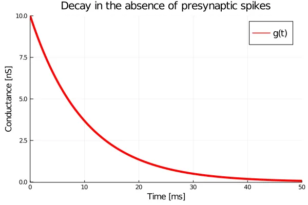
The ISED model assumes that a pre-synaptic spike causes an instantaneous increase in conductance, which subsequently decays with time. If the conductance is denoted as , and it decays with a time-constant , the conductance dynamics in the absence of any presynaptic spikes can be expressed very simply:

Thus, the higher the conductance, the faster it decays. The stable node at ensures that all trajectories decay exponentially to this fixed-point - i.e., given sufficient time, the electric flux all but disappears. In the following graph I plot the scenario where a synapse with has a conductance of about at , i.e., . We see that in (i.e., ), the conductance has already decayed to almost zero.

Notice that we have not talked about any perturbations yet. This is where the ‘I’ from ISED comes in. Each pre-synaptic spike is modelled as an instantaneous increase in the conductance. A more complete description of the behaviour of the synapse is:

Here, is the timing of the -th presynaptic spike, is the amplitude of the perturbation caused by this -th spike, and is the Dirac delta function. Such equations are quite common in systems which jump about in phase space due to sharp external inputs. In the case of our ISED synapse, we could simply interpret it as: whenever a pre-synaptic spike occurs, the conductance rises instantaneously by a certain amount, and the decay starts all over again. More rigorously one could write this jump in conductance as:

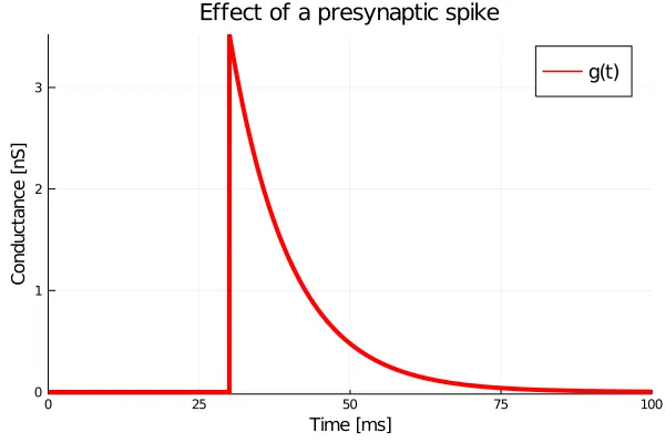
where . Below, I show the results of a simulation where an ISED synapse at rest, i.e., , receives a pre-synaptic spike at about . Notice how there is no delay and the conductance shoots up immediately to about (the exact value is immaterial here), before decaying back to .

An important property of ISED synapses is that after the instantaneous jump (at say, ), the time-course of the response no longer depends on the amplitude of this jump. This gives the system a sort of ‘memorylessness’. In this memoryless system, the multiplicative exponentials in the solution to equation can be stacked one after the other in time. Below, I show a simulation where a synapse with receives a pre-synaptic spike at about , followed by a quick volley of four spikes occurring between and .

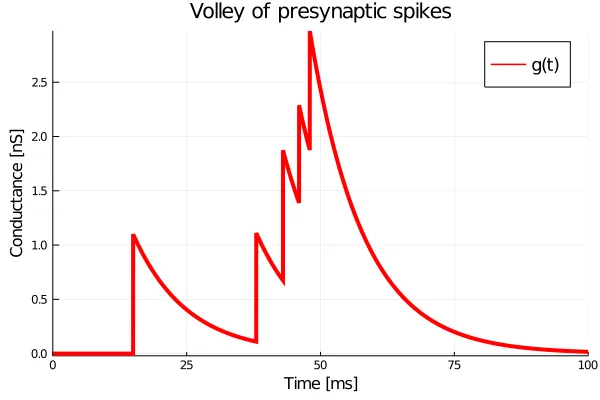
As expected, each jump simply resets the time-course of the response and the conductance continues to decay with a time-constant . However, real synapses cannot be instantaneous, because electric flux cannot move at infinite speed. A first approximation to a realistic synaptic transfer function will be discussed in the next article.y resets the time-course of the response and the conductance continues to decay with a time-constant . However, real synapses cannot be instantaneous, because electric flux cannot move at infinite speed. A first approximation to a realistic synaptic transfer function will be discussed in the next article.